			GASLAB: GAS IN A BOX

WHAT IS IT?
-----------
	This program simulates the behavior of gas molecules
in a closed container. It was one of the original CM StarLogo
applications (under the name GPCEE) and is now ported to
StarLogoT as part of the Connected Mathematics "Making Sense
of Complex Phenomena" Modeling Project.

	The Gas-in-a-Box model is the first in a collection
of GasLab models that all use the same basic rules for
expressing what happens when gas molecules collide. Each of
the GasLab models has different features in order to show
different aspects of the behavior of gases.

	Molecules are modeled as perfectly elastic particles
with no internal energy except that which is due to their
motion. Collisions with the walls and between molecules are
elastic.  Particles are colored according to speed -- blue
for slow, green for medium, and red for high speeds.

	The exact way two molecules collide is as follows:
1.  Two turtles "collide" if they find themselves on the
same patch.
2.  A random axis is chosen, as if they were two balls that
hit and this axis were the line connecting their centers.
3.  They exchange momentum and energy along that axis,
according to the conservation of momentum and energy.
This calculation is done in the center of mass system.
4. Each turtle is assigned its new speed, energy, and
heading.
5.  If a turtle finds itself on or very close to a wall of
the container, it "bounces" -- that is, reflects its
direction and keeps its same speed.

The creation and use of the GasLab modeling toolkit is
described in detail in the two papers listed at the end of this
info window.

HOW TO USE IT
-------------

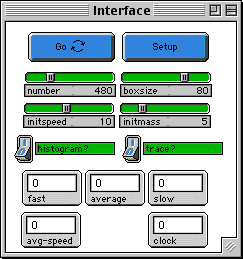
SETUP: puts in the initial conditions you have set with
the sliders.  Be sure to wait till the Setup button stops
before pushing go.
GO: runs the code again and again.  This is a "forever"
button.
NUMBER:the number of gas molecules.
INITSPEED:  the initial speed of each molecule -- they
all start with the same speed.
INITMASS: the mass of each molecule.

HISTOGRAM?: If this equals 1, the histograms are plotted
every 6 ticks.  This plotting frequency can be modified
with the variable "plotfrq".
TRACE?: Stamps the path of one individual molecule. This
path fades in time to make the screen less cluttered.

FAST, AVERAGE, SLOW MONITORS: numbers of molecules with
different speeds: fast (red), average (green), and slow
(blue).
AVG-SPEED:  average speed of the molecules.
CLOCK:  number of ticks that have run.

GRAPHS:
  ENERGY HISTOGRAM (1): the distribution of energies of
all the molecules, calculated as  m*v*v/2.
The yellow line is the initial value.
  SPEED HISTOGRAM (2): speed distribution of all the
molecules.  The yellow line is the initial value.
The running average value is shown in the "avg-speed"
monitor.
The red and blue lines mark the limits of "fast" and "slow"
molecules.  All the molecules between these two lines are
green (average speed).
  SPEED COUNTS (3): the numbers of red, green, and blue
molecules as time goes by.

	Initially, all the molecules have the same speed
but random directions. Therefore the first histogram plots
of speed and energy should show sharp spikes. The yellow
line on the graph marks the initial speed. As the
molecules repeatedly collide, they exchange energy and head
off in new directions, and the speeds are dispersed -- some
molecules get faster, some get slower.

RUNNING the MODEL
-----------------

        THINGS TO NOTICE
        ----------------

What is happening to the relative numbers of molecules of
different colors?  Does this match what's happening in the
histograms? Why are there more blue molecules than red ones?

Can you observe collisions and color changes as they happen?
For instance, When a red molecule hits a green molecule,
what color do they each become?

Why does the average speed (avg-speed) drop?  Does this
violate conservation of energy?

The molecule histograms quickly converge on the classic
Maxwell-Boltzmann distribution.  What's special about these
curves?  Why is the shape of the energy curve not the same
as the speed curve?

Watch the molecule whose path is traced in yellow. Notice
how the path "wraps" the screen. Does the trace resemble
Brownian motion?  Can you recognize when a collision
happens?  What factors affect the frequency of collisions?
What about the "angularity" of the path?   Could you get
it to stay "local" or travel all over the screen?

In what ways is this model an incorrect idealization of the
real world?

In this model, molecules bounce off the walls like elastic
tennis balls.  Is this equivalent to an "insulated box"?
What happens at the walls of a REAL insulated box?

If all the molecules are identical at the start, why don't
they stay that way?  How could a speed distribution arise
from simple collisions of particles with equal mass?

        THINGS TO TRY
        -------------

Try different initial settings, especially the extremes.
Are the histograms different?  Does the trace pattern change?
Compare the amount of change in average speed (avg-speed).

Try molecules with more than a single mass,using a
StarlogoT command.

Try other initial speed distributions.

Set all the molecules in the center of the box or with the
same heading - what happens? Is this a physical possibility?

Set up only two molecules to collide head-on.  This may help
to show how the collision rule works.  Remember that the
axis of collision is being randomly chosen each time.

Are there other interesting quantities to keep track of?

Figure out how many molecules there REALLY are in a box this
size -- say a 10-cm cube.  Look up or calculate the REAL
mass and the REAL speed of a typical molecule. When you
compare those numbers to the ones in the model, are you
surprised this model works as well as it does?  What
physical phenomena might be observed if there really were
a small number of molecules in the space around us?

EXTENDING THE MODEL
-------------------

In what ways is this idealization different from the
idealization that is used to derive the Maxwell-Boltzmann
distribution? Specifically, what other code could be used
to represent the two-body collisions of molecules?

What happens if there are molecules of different masses?
(See Two Gas model.)

How would you calculate pressure in the box?  (See Piston
models.)

Could you find a way to measure or express the "temperature"
of this imaginary gas?  Try to construct a thermometer.

What would happen if you introduced a piston into the box
that could change the volume of the gas? (see "Piston"
models)

What happens if the collisions are non-elastic?

What happens if you introduce heat and/or cold plates?

How does this 2-D model differ from the 3-D model?

What if some of the molecules had a "drift" tendency -- a
force pulling them in one direction?  Could you develop a
model of a centrifuge, or charged particles in an electric
field?

Find a way to monitor how often molecules collide, and how
far they go between collisions, on the average.  The latter
is called the "mean free path".  What factors affect its
value?  How is this related to diffusion of, say, a smell
in a room?

If MORE than two molecules arrive on the same patch, the
current code says they don't collide.  Is this a mistake?
How does it affect the results?

Is this model valid for fluids in any aspect?  How could
it be made to be fluid-like?

STARLOGOT FEATURES
-----------------
During each tick, each turtle checks many times to see if
it has collided.

Notice the use of the command histogram-turtles in
histo-speed and histo-energy.

Notice how collisions are detected by the turtles and how
the code guarantees that the same two particles do not
collide twice.  What happens if we let the patches detect
them?

You can find specific values on the graphs by clicking the
mouse on the point whose value you would like.  The
coordinates of that point are shown in red if you're right on
the line, and blue otherwise.

REFERENCES
-----------

Wilensky, U. (in press). GasLab-an Extensible Modeling Toolkit
for Exploring Micro- and Macro- Views of Gases. In Roberts, N.
, Feurzeig, W. & Hunter, B. (Eds.) Computer Modeling and
Simulation in Science Education. Berlin: Springer Verlag.
http://www.ccl.tufts.edu/cm/papers/gaslab/index.html

Wilensky, U., Hazzard, E., & Froemke, R. (1999). GasLab - an
Extensible Modeling Toolkit for Exploring Statistical
Mechanics.  In Proceedings of the 7th Annual European Logo
Conference, August 1999, Sofia, Bulgaria.
http://www.ccl.tufts.edu/cm/papers/gaslab2/index.html
