WHAT IS IT?
-----------
This model illustrates the Law of Supply and Demand which is the fundamental tool
of economic analysis. The law of supply and demand states that, in a free market,
the price of a good will move to a point where the quantity supplied and the
quantity demanded are equal. This point is known as 'equilibrium'. In theory, if
the functions determining the quantity supplied at a given price (the supply
function) and the quantity demanded at a given price (the demand function) are
well defined - as in this model - this law works very well. In practice, markets
tend to be much more complicated and application of the law is not as
straightforward. Real markets occasionally will disobey it, as there can be market
gluts and shortages, but for the most part the law of supply and demand is a fair
economic generalization.
This model demonstrates both the theory behind the law of supply and demand and
how the law is realized in a theoretical market of buyers and sellers. The supply
and demand functions can be computed and plotted ahead of time, thus yielding an
equilibrium price as predicted by theory. The model can then be run, and from the
interactions between the buyers and sellers we see that in trying to maximize
profit the sellers eventually narrow in on the equilibrium price.
As the model is run it will iteratively cycle through two phases: an interaction
phase (known as a 'round'), in which buyers visit sellers and purchase goods, and
a adjustment phase, in which prices and inventories are redetermined and buyer and
seller variables are reinitialized. It is important to note the activity of the
buyers and the sellers in one cycle in order to understand how an equilibrium
price is eventually reached.
The buyers buy one unit, if they are able to, each round. They will visit up to
ten different sellers searching for a price at which they can afford to buy the
good. If the seller has inventory on the item and the buyer has enough money, then
the purchase is made. The money in the buyers' wallets is equal to their income
per round, a random amount between five and fifty that is determined for each
buyer when the SETUP button in pressed. This money does not accumulate from round
to round, and so a buyers will always begin every round with the same amount of
money.
Sellers each have an individual price at which they will sell one unit of their
inventory. This price is initialized randomly to a value between 5 and 50 when the
SETUP button is pressed. New inventory is computed after each round by taking the
selling price and dividing it by the cost price (or wholesale price) of the good,
which is set as a constant at 5 dollars. This amount is then rounded down, and
added to any existing inventory (left over from the previous rounds). For example,
a seller with a price of 27 will restock 5 units (27/5 rounded down to 5) to the
existing inventory. When SETUP is pressed, a seller initialized with a price of 27
will begin the simulation with an inventory of 5 units.
A simple heuristic is used for the sellers to approximate the price at which their
profit will be maximized. If the sales from the previous round met or exceeded a
seller's inventory, then there is a ten percent chance that the seller will raise
the price. If the sales were less than the inventory, then the seller will lower
the price by one. In the real world such a strategy might not be very feasible,
but it is important to note that there is no magic formula for determining
pricing. As with real companies, sellers in this model have no access to an actual
demand function on which to base their decisions (sellers can NOT simply calculate
the equilibrium price!). This would require 'global' information about the market,
but sellers in this model have only the 'local' information about their individual
sales and inventories to work with. (Note that through surveys and polling of
potential customers, large companies today often do try to determine general
information about their market. However, as this model demonstrates, global
information about the market is not necessary for equilibrium to be reached.)
Before or during the running of the model, a plot of the supply and demand
functions can be made to predict the equilibrium price (using COMPUTE-CURVES). The
demand function is determined by calculating the total number of buyers with
incomes greater than or equal to each corresponding price on the y-axis. This is
the total quantity that will be sold at that price. The supply function is equal
to the total amount of inventory that will be available in the market if every
seller sets their price to the corresponding price on the y-axis. This is the
total quantity that will be produced at that price. The price at which these
curves intersect is the equilibrium price. Because of rounding down in
determination of supply at a given price, the supply function is actually a step
function - it has been smoothed to simplify interpretation.
There are many possibilities to extend this model beyond its basic framework to
provide an analysis of different economic factors. The law of supply and demand
can be used, among other options, to analyze unemployment, the value of the dollar
overseas, international trade, and environmental protection. See the 'EXTENDING
THE MODEL' section for a list of ideas.
HOW TO USE IT
-------------
The number of buyers and sellers can be adjusted on the interface panel. Choose a
ratio between the number of buyers and the number of sellers, or to start off try
a ratio of one hundred buyers to twenty sellers. Press the SETUP button, and then
press GO. Buyers are in green, Sellers are in blue. The average price after each
round is plotted over time on the second plot window. The first plot window is
used to predict what the equilibrium price will be based on the supply and demand
functions.
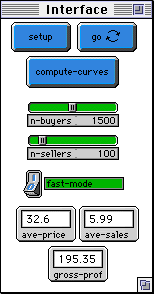
INTERFACE ITEMS:
SETUP: resets the simulation according to new settings
GO: runs the simulation.
COMPUTE-CURVES: computes and plots the supply and demand curves for the current
run (plot-window 2). the intersection of the these curves is the predicted
equilibrium price.
N-BUYERS: sets the number of buyers to create when RESET is pressed. Has no
effect during a simulation.
N-SELLERS: sets the number of sellers to create when RESET is pressed. Has no
effect during a simulation.
FAST-MODE: turns on/off the graphic display of the buyers entering the
marketplace. The simulation runs faster with the graphics turned off.
AVE-PRICE: shows the average selling price of all of the sellers.
AVE-SALES: shows the average number of sales for all of the sellers.
GROSS-PROFIT: shows the average gross-profit for all of the sellers.
PLOTS:
PREDICTED-EQUILIBRIUM-PRICE: To activate this plot, press the COMPUTE-CURVES
button. Shown in blue is the supply-function for the sellers in the
simulation. That is, corresponding to each quantity (on the x-axis)
is the price they are willing to sell one unit for. The supply function does
not change from run to run or as the settings are changed. Shown in green is
the demand function for the buyers in the simulation. That is, corresponding
to each price (on the y-axis) is the number of buyers who are willing to buy
at that price. As each buyer buys only one unit per round in this model, this
is equivalent to the quantity that will be bought at that price. The
demand function changes as the settings are changed and, because income is set
randomly for each buyer when the reset button is pressed, it will typically
shift slightly from between runs with the same settings. The price at which
the two curves intersect is known as the equilibrium price, which will be just
below the number indicated on the top of the y-axis. As the supply and demand
functions do not change during a simulation, sellers should - in theory -
maximize gross-profit by selling at the equilibrium price.
PRICE-OVER-TIME: tracks the average selling price over time.
SALES-OVER-TIME: tracks the average quantity sold (per seller) over time.
GROSS-PROFIT-OVER-TIME: tracks the average gross-profit (per-seller) over
time.
THINGS TO TRY
-------------
Try varying the ratio of buyers to sellers. What is the relation between this
ratio and the average price of the good?
What happens to the price when there is a scarcity or an abundance of the good?
After pressing SETUP, press COMPUTE-CURVES and look at the predicted equilibrium
price. Now run the model. Does the average price generated from the model fit the
prediction. Under what circumstances will the prediction fail? Why?
EXTENDING THE MODEL
-------------------
The demand and supply curves in this model are linear. This is because sellers
have no direct control over the quantity they stock - the amount of inventory is a
determinate, linear function of their selling price. Some things you can do to
change this: (1) Introduce a variable inventory so that sellers can control both
price AND quantity of inventory. (2) Make the mapping from price to amount of
inventory non-linear. Often supply functions (also demand functions) are modeled
as quadratic curves, as efficiency or interest in producing the good may rise or
fall with the selling price.
Introduce multiple goods into the system. Have buyers with variable demand for the
different goods.
This model doesn't take geography into account - set up conditions so that
different areas of the screen lead to buyers and sellers with different
characteristics. One way to this would be to have sellers 'forage' for goods
instead of purchasing them wholesale. Goods could sprout from patches, and various
areas could have different growth characteristics or grow different products. What
kinds of regional differences can you get to emerge (i.e. lower priced areas,
high-income areas)?
Test the pricing strategy of the sellers - are they maximizing their gross-profit?
Why do you think that the price setting heuristic works as well as it does?
Discover and implement a better price-setting strategy - perhaps one that isn't a
probabilistic heuristic, but that has explicit rules.
Where do the sellers' profits go? Have a model that conserves the total amount of
money in the system and/or resources in the system to demonstrate a true flow of
goods.
How would government policies affect the model? What happens when a sales tax is
imposed? What is the effect of a federally imposed price floor, such as the
minimum wage price on labor? Play the role of government and test your policies on
the model.
Can variables be introduced which take into account the externalities of
production, i.e. pollution?
The model can be used more generally to consider international trade between an
importer and an exporter. How do tariffs and quotas affect the model? What are the
benefits to the nation that imports?